EA Lidar WCS — elevation + analysis#

Fetch a small British National Grid window from the Environment Agency Lidar composite DTM (WCS), plot elevation, and summarise the distribution.

Uses WCSConfig.for_ea_dsp (AIMD under a hard ceiling, pressure circuit breaker). Keep large cold mosaics at or below the preset ceiling — higher limits can trip gateway pressure.

Code#

from tilearray import compute_with_policy, create_array
from tilearray.service import WCSConfig
from tilearray.types import CRS, Format

wcs_url = (
    "https://environment.data.gov.uk/spatialdata/"
    "lidar-composite-digital-terrain-model-dtm-1m/wcs"
)
coverage_id = (
    "13787b9a-26a4-4775-8523-806d13af58fc__Lidar_Composite_Elevation_DTM_1m"
)

config = WCSConfig.for_ea_dsp(
    wcs_url,
    coverage_id=coverage_id,
    crs=CRS.EPSG_27700,
    output_format=Format.GEOTIFF,
    chunk_size=(64, 64),
    resolution=(1.0, 1.0),
)

# ~256 m OSGB window
bbox = (431900.0, 382700.0, 432156.0, 382956.0)

da = create_array(config, bbox, CRS.EPSG_27700)
elevation = compute_with_policy(da)  # match Dask workers to fetch ceiling
print(elevation.shape, float(elevation.mean()))

create_array stays lazy until compute. For multi-tile mosaics, prefer tilearray.compute_with_policy() over plain .compute().

Result#

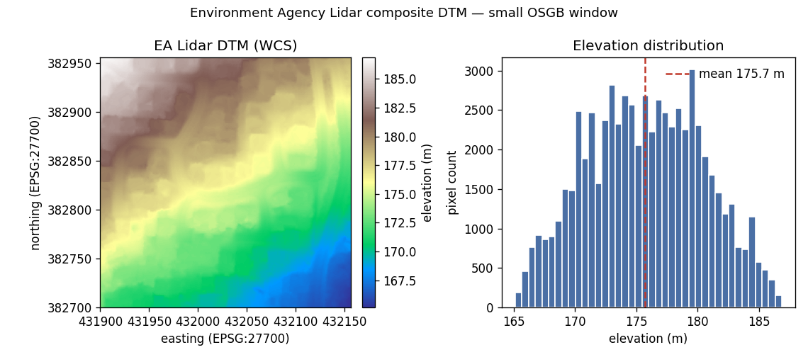
EA Lidar elevation map and histogram for a small OSGB window

Example stats for this window: shape (256, 256), mean elevation about 176 m (see histogram). More public endpoints: Example sources.